

Brain Tumor Detection with OpenCV
With the rapid advancement of current technology, brain tumor detection is an important and developing field that has drawn prime attention from the scientific community. A brain tumor is an uncontrolled development of brain cells from the patients with brain cancer. As we are concerned about, early diagnosis of brain tumor plays an essential role in how the patient will be treated as well as their survival rate. According to current medical reports, there are a variety of brain tumor forms with unique properties and respective therapies. Hence, manual brain tumor detection is complicated and vulnerable to human error. As a result, machine-learning assisted diagnosis with efficient algorithm and high precision is highly demanded and currently developed by several doctors, bioinformaticians and computer scientists. In this project, I used the image segmentation from OpenCV library and two algorithms of convolutional neural networks, specifically ResNet50 and VGG19, which have been widely used in the medical field for the past few years. In this paper, I will give an illustration of how I process the image data and build the ML model by implementing ResNet50 and VGG19.
To begin with, I chose a dataset that have 3002 pictures in total from Kaggle.com. Half of them is the brain with tumor and half is a healthy brain. The dataset has other files such as prediction, testing, training,…, which I did not use. So, for my dataset, it has two folder, no and yes. “No” contains the images of non-tumor brains and “Yes” contains the images of tumorous brains. Each folder has 1500 images, which is sufficient to create a good model. I previously had a dataset but it was small so I changed to this one. The pictures below demonstrate the basic difference between non-tumor and tumorous brains.


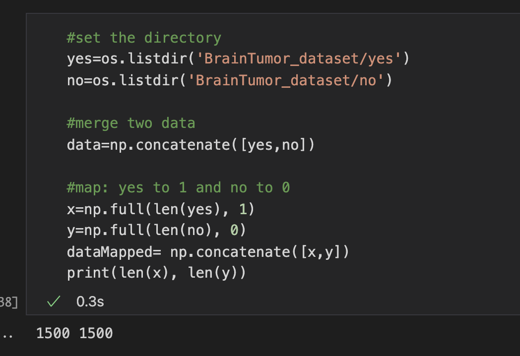
Before going to preprocess the data, I map the yes images to 1 and no images to 0 and create a simple array. This array, with actual correct labels, will be used for the model to compare with the training data.
The next step is data preprocessing, which I resized all the images to a certain dimension (200x200) and then append to an array while saving those images in the dataset.

Following this, I wrote a function called imageCrop, which takes in the image file and crops the background, only leaving the brain image with the rectangular background. This was a new experience for me as a newbie to computer vision. The function has five primary steps and uses methods from OpenCV, which is a library of Python bindings designed to solve computer vision problems. The first step was to convert the image to gray scale and blur it to reduce high frequency noise to make the contour detection process more accurate.

Figure 1: Change to grayscale
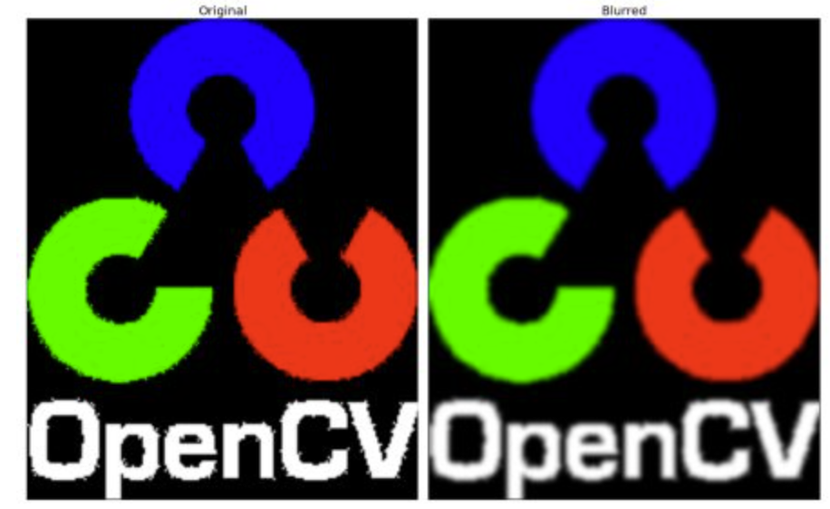
Figure 2: Gaussian Blur
The second step is to change the pixels to make the image easier to analyze, which is to binarize it with black background and white image). I used erode and dilate methods, which are to remove the pixels of the boundaries of the image and add pixels to the boundaries of the image. This sounds like that erosion and dilation are opposite against each other (not commutative, mathematically speaking). In fact, their algorithms work quite differently and they are useful tools for programmers to increase the accuracy of the model, falling under the name of morphological operations, which are used across mathematics, physics,…


Figure 3: Normal – Erosion - Dilation
The third step is to find the contour of the image, which is to spot the line that goes across the boundary of the image (white-colored against the black background). At the same time, I removed false positives and noises on the image. Then I found the biggest area of the contours

Figure 4: findContours()
The fourth step is to find the extreme outer coordinates of the picture using the maximum positions found in the previous step.

Figure 5: dark blue (top), light blue (bottom), yellow (right), red(left)
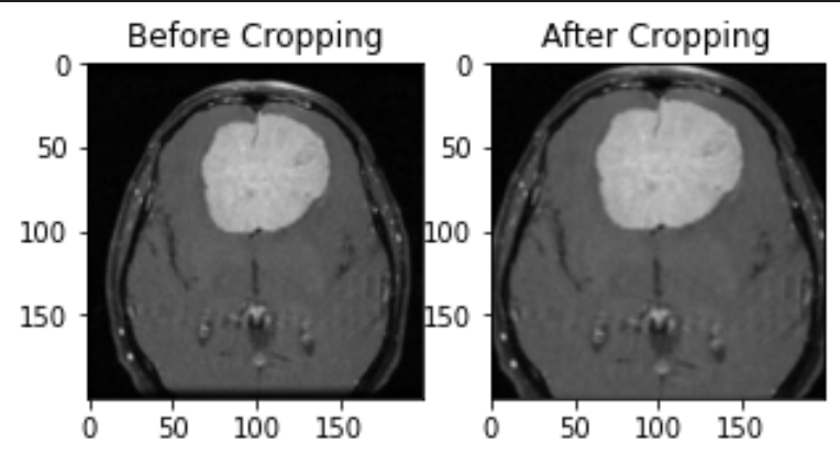
The last step is to resize the image. Here is when I applied the function to the dataset
After cropping, I moved to normalize the data and split the data into training, testing, and validation ( the ratio is 70% - 15% - 15%). I have the preprocessData(x,y), which preprocesses the input for me and makes the input suitable for the Resnet50 implementation, which is where I realized I need to use a separate dataset for CGG19 but I did not have time so I just went ahead and use the same for those algorithms. After this step, I did data augmentation, which is to increase the amount of data by adding slightly modified copies of already existing data to regularize and reduce overfitting. I created the augmented dataset for each type (train, test, and val). However, I did not use these because the model works fine without it.
The most important step is to implement two CNN algorithms. I will give some introductions to these two algorithms. On the one hand, ResNet50, or Residual Neural Network was introduced in 2015, featuring heavy batch normalization and skip connections. This technique enabled to train a neural network with 152 while having lower complexing than VGG. It has achieved 3.57% error, which beats human-level performance. This is really impressive to know when I found out about this algorithm. On the other hand, VGGNet was introduced in 2014 and consists of 16 convolutional layers with very uniform architecture. It is currently the most preferred choice to extract features from images. However, VGGNet consists of 138 million parameters, which makes it time-consuming and computationally intensive for the implementation process.
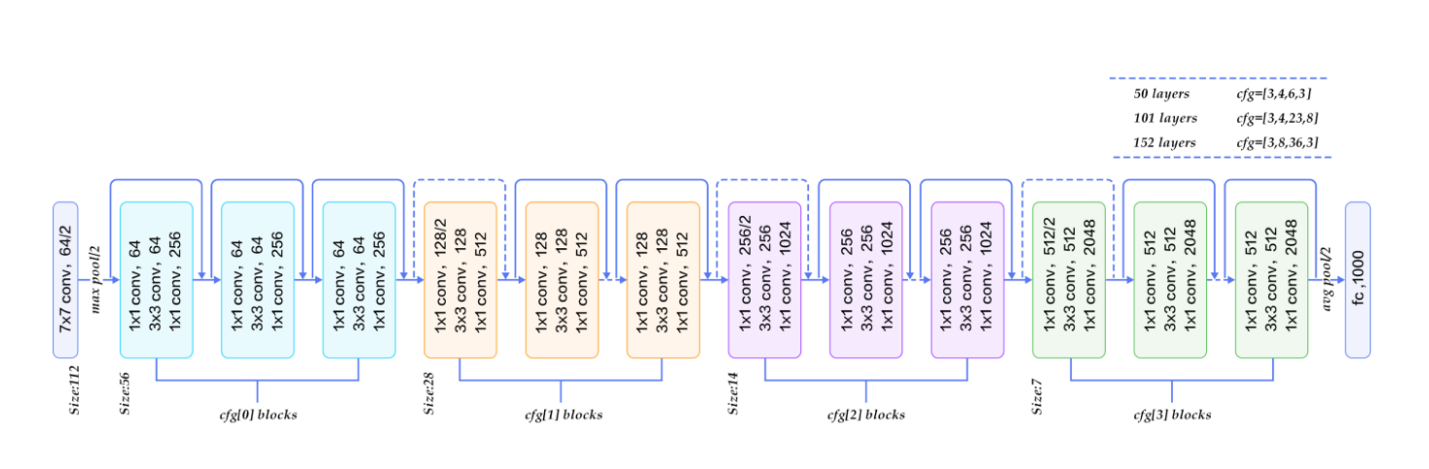
Figure 6: ResNet Architecture
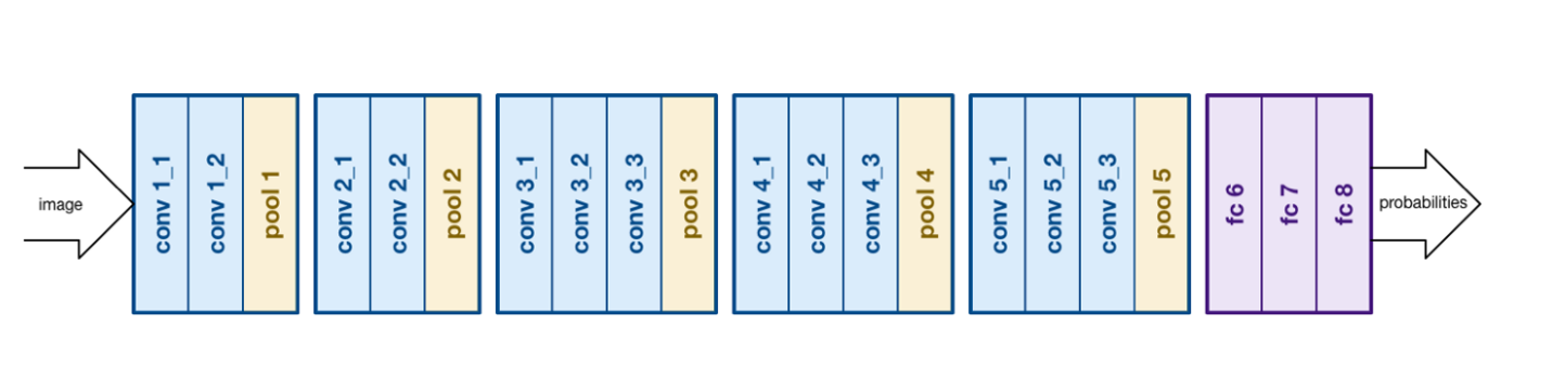
Figure 7: VGGNet Architecture
To go into details of Resnet50, in the process, I used Sequential model from the tensorflow.keras library and applied relu as my activator function for my input and softmax as my activator function for my output (3 dense layers of relu and 1 dense layer of softmax). For the compilation process, I used adam as my optimizer with checkpoint and early stopping to fit the dataset into Resnet algorithm. The fitting process takes 53 minutes and 23.6 seconds (batch size is 32 and epoch is 20). At epoch =18, the accuracy starts to peak and decrease, which means the model cannot generalize any more and will lead to overfitting, according to bias-variance trade-off. The accuracy goes up really fast and so is the value accuracy. The test accuracy was 0.842 and the precision was 0.841.

(Accuracy Graph of Resnet 50)

The graph above is the confusion matrix that describes how non-tumor and tumor images were predicted correctly by the model.
To go into details of VGG19, I used relu as the activator function for both of my input and output, which actually caused inaccuracy in the fitting process I believe. I changed activator function for the output to sigmoid and softmax, but both raised the error on binary classes, which I encountered through out the implementation only to realize that I had to use a different training and testing set because ResNet50 tuned my dataset, making it unfit for VGG19. However, I managed to fit the data with binarycrossentropy and SGD as the optimizer, which was really time-consuming with 112 steps for each epoch. This time, the batch size is only 16 and the number of epoch is 10, but it took 63 minutes and 51.8 seconds to run. This implies that VGG19 is really computationally intensive. I used a MacBook Pro 16 (2019) but it drained up the laptop’s battery very fast. The accuracy and val_acc almost kept constant throughout the fitting process (approximately 0.7543 and 0.9). The test accuracy was 0.898, which is a little lower than Resnet50 but still very impressive. Because the dataset was not tunned for VGG19, I was not able to retrieve precision score and recall score for this model. Python would raise “Classification metrics can’t handle a mix of multilabel-indicator and binary targets, which I see a common theme of error in using tensorflow and keras.
I tried to graph images of brain with tumor and brain without but I got into an error “only integer scalar arrays can be converted to a scalar index”, which probably is the result of incompatibility of tuned dataset for Resnet50. For the future prospect, I will try to reserve a different dataset for VGG so that I can perform accuracy metrics on the model.
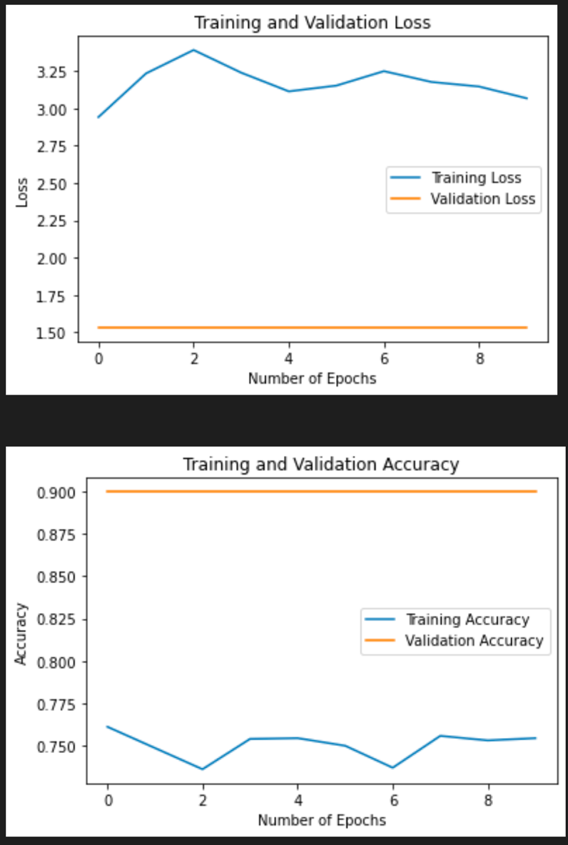
(Accuracy Graph of VGG19)
In conclusion, this project was a challenge for me. I wanted to get my foot in the medical field and it was not easy as I never learn Biology in English before. The errors were quite frustrating as this field is still pretty new so there are not much of resources out there to look for. Also, the fitting process was really time-consuming. Before the finalization, the number of epoch in VGG was 100 and I let my laptop run overnight but it could not finish it yet. So I reduced it bit by bit. But realizing my mistake from the dataset, I reduced it to 10 and the batch size to 16. For Machine Learning project, I only used a very simple version of NN which is the Multilayer Perceptron Classifier. But for this one, I really digged deep into the very idea of convolutional neural network and deep learning, which I found quite interesting and hopefully I can work on some similar projects in the future.
(I included my github repos and made it public so you can take a look at my actual code)
Reference:
https://www.kaggle.com/ahmedhamada0/brain-tumor-detection (dataset)
https://github.com/leestorm4520/DataScience_BrainTumorDetection.git (github repos)
https://www.jeremyjordan.me/convnet-architectures/
https://stackoverflow.com/questions/56781635/find-extreme-outer-points-in-image-with-python-opencv
https://docs.opencv.org/3.4/index.html
https://github.com/MohamedAliHabib/Brain-Tumor-Detection
https://github.com/slowy07/brain-tumor-detection
https://github.com/reasad/Brain-Tumor-Detection
https://github.com/PritomDas/Brain-Tumor-Detection-with-Deep-Learning
https://medium.com/@kenneth.ca95/a-guide-to-transfer-learning-with-keras-using-resnet50-a81a4a28084b
https://www.mathworks.com/help/images/morphological-dilation-and-erosion.html

